


Supervised Learning with scikit-learn - Part 4
Chapter 4 - Preprocessing and Pipelines
Learn how to impute missing values, convert categorical data to numeric values, scale data, evaluate multiple supervised learning models simultaneously, and build pipelines to streamline your workflow!
import pandas as pd
import numpy as np
import warnings

pd.set_option('display.expand_frame_repr', False)

warnings.filterwarnings("ignore", category=DeprecationWarning)
warnings.filterwarnings("ignore", category=FutureWarning)
Preprocessing data
scikit-learn requirements:
- Numeric data
- No missing values
- With real-world data:
- This is rarely the case
- We will often need to preprocess our data first
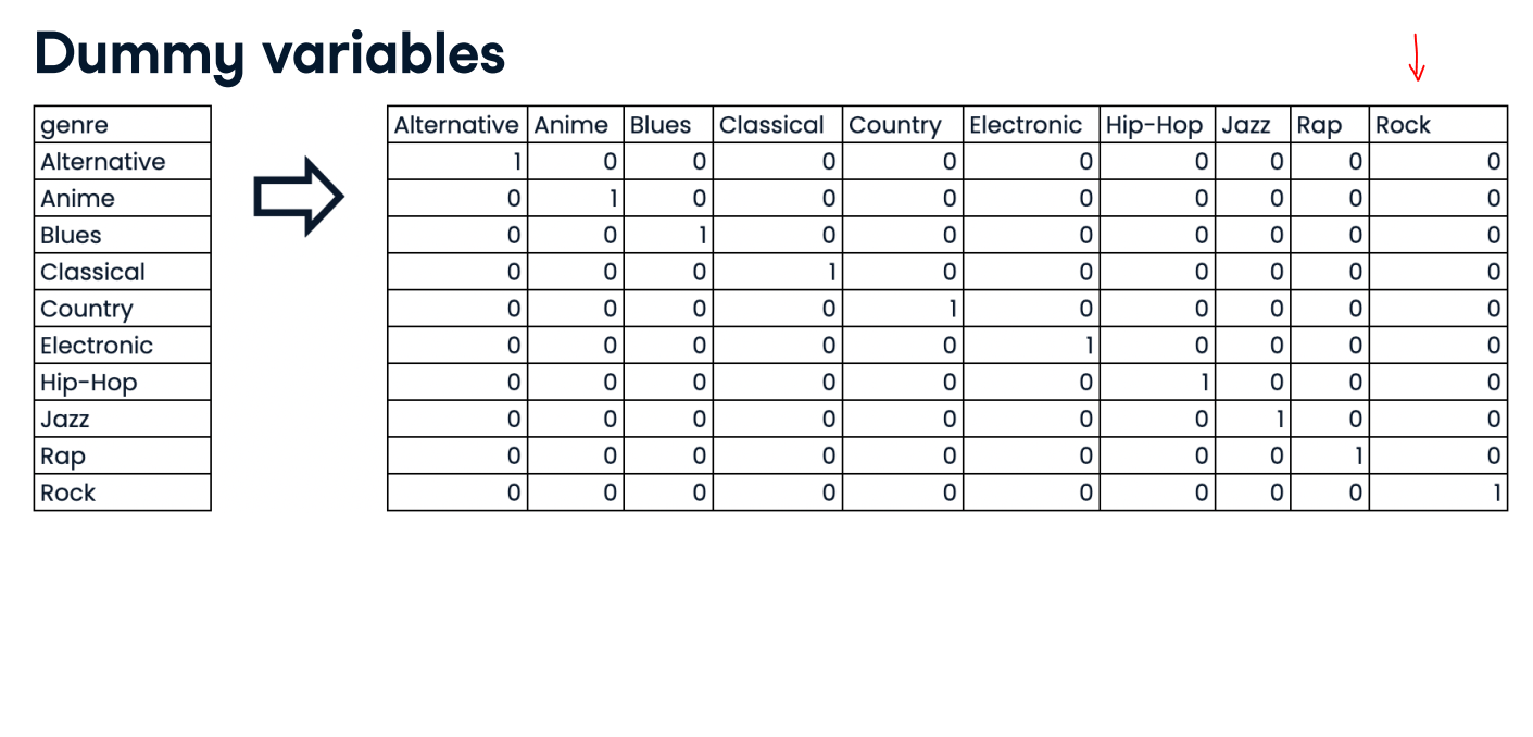
Example of Dealing with categorical features
- scikit-learn will not accept categorical features by default
- Need to convert categorical features into numeric values
- Convert to binary features called dummy variables:
- 0: Observation was NOT that category
- 1: Observation was that category
music_clean_df = pd.read_csv('./datasets/music_clean.csv',index_col=[0])
display(music_clean_df.head())
cols = music_clean_df.columns.to_list()
print(cols)
print(music_clean_df.info())
music_df_full = pd.read_csv('./datasets/music_genre.csv',index_col=0)
music_df_full.rename(columns={'music_genre': 'genre'}, inplace=True)
music_df_full = music_df_full.loc[music_df_full['tempo'] != '?']

music_df = music_df_full[cols].sample(1000)
music_df['tempo'] = music_df['tempo'].astype(float)

music_df.reset_index(drop=True, inplace=True)

print(music_df.info())
display(music_df.head())
music_dummies = pd.get_dummies(music_df['genre'], drop_first=True)
print(music_dummies.head())
music_dummies = pd.concat([music_df, music_dummies], axis=1)
music_dummies = music_dummies.drop("genre", axis=1)
music_dummies = pd.get_dummies(music_df, drop_first=True)
print(music_dummies.columns)
from sklearn.model_selection import cross_val_score, KFold, train_test_split
from sklearn.linear_model import LinearRegression


X = music_dummies.drop("popularity", axis=1).values
y = music_dummies["popularity"].values
X_train, X_test, y_train, y_test = train_test_split(X, y, test_size=0.2, random_state=42)

kf = KFold(n_splits=5, shuffle=True, random_state=42)
linreg = LinearRegression()
linreg_cv = cross_val_score(linreg, X_train, y_train, cv=kf,
scoring="neg_mean_squared_error")
print(np.sqrt(-linreg_cv))
Creating dummy variables (Exercise)
Being able to include categorical features in the model building process can enhance performance as they may add information that contributes to prediction accuracy.
The music_df dataset has been preloaded for you, and its shape is printed. Also, pandas has been imported as pd.
Now you will create a new DataFrame containing the original columns of music_df plus dummy variables from the "genre" column.
Instructions:
- Use a relevant function, passing the entire music_df DataFrame, to create music_dummies, dropping the first binary column.
- Print the shape of music_dummies.
music_dummies = pd.get_dummies(music_df, drop_first=True)

# Print the new DataFrame's shape
print("Shape of music_dummies: {}".format(music_dummies.shape))
As there were ten values in the "genre" column, nine new columns were added by a call of pd.get_dummies() using drop_first=True. After dropping the original "genre" column, there are still eight new columns in the DataFrame!
Regression with categorical features (Exercise)
Now you have created music_dummies, containing binary features for each song's genre, it's time to build a ridge regression model to predict song popularity.
music_dummies has been preloaded for you, along with Ridge, cross_val_score, numpy as np, and a KFold object stored as kf.
The model will be evaluated by calculating the average RMSE, but first, you will need to convert the scores for each fold to positive values and take their square root. This metric shows the average error of our model's predictions, so it can be compared against the standard deviation of the target value—"popularity".
Instructions:
- Create X, containing all features in music_dummies, and y, consisting of the "popularity" column, respectively.
- Instantiate a ridge regression model, setting alpha equal to 0.2.
- Perform cross-validation on X and y using the ridge model, setting cv equal to kf, and using negative mean squared error as the scoring metric.
- Print the RMSE values by converting negative scores to positive and taking the square
from sklearn.linear_model import Ridge
# Create X and y
X = music_dummies.drop(['popularity'], axis =1).values
y = music_dummies['popularity'].values

# Instantiate a ridge model
ridge = Ridge( alpha=0.2)

# Perform cross-validation
scores = cross_val_score(ridge, X, y, cv=kf, scoring="neg_mean_squared_error")

# Calculate RMSE
rmse = np.sqrt(-scores)
print("Average RMSE: {}".format(np.mean(rmse)))
print("Standard Deviation of the target array: {}".format(np.std(y)))
Great work! An average RMSE of approximately 9.4 is lower than the standard deviation of the target variable (song popularity), suggesting the model is reasonably accurate.
Dropping missing data
Over the next three exercises, you are going to tidy the music_df dataset. You will create a pipeline to impute missing values and build a KNN classifier model, then use it to predict whether a song is of the "Rock" genre.
In this exercise specifically, you will drop missing values accounting for less than 5% of the dataset, and convert the "genre" column into a binary feature.
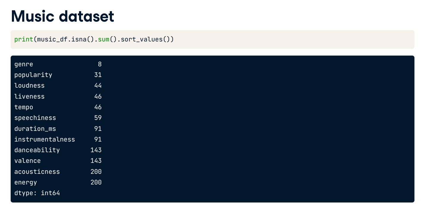
Instructions:
- Print the number of missing values for each column in the music_df dataset, sorted in ascending order.
print(music_df.isna().sum().sort_values())
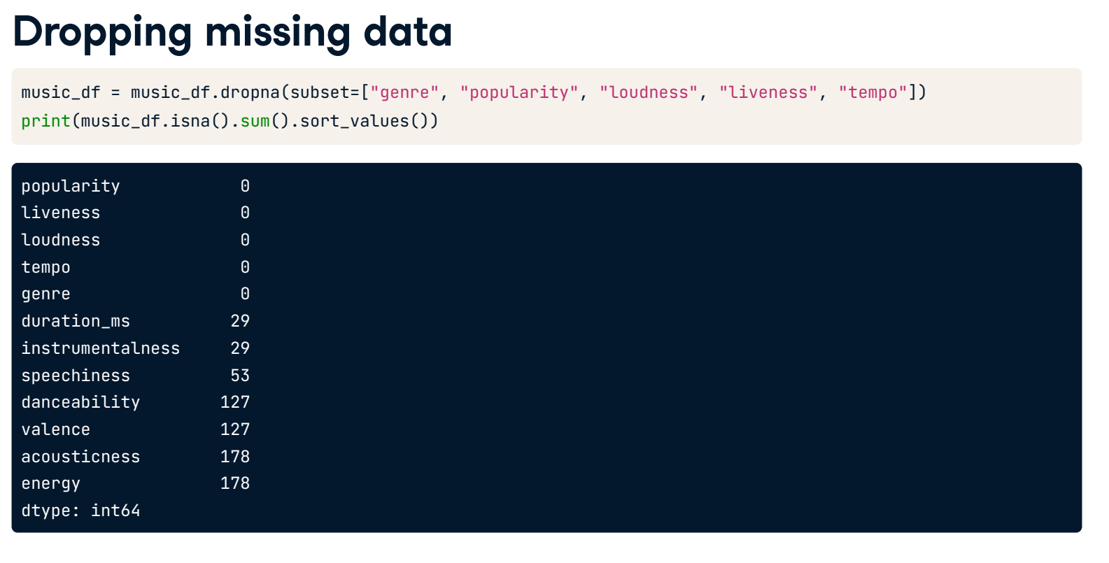
- Remove values for all columns with 50 or fewer missing values.
print(music_df.isna().sum().sort_values())
lessthan50NanCols = [i for i in music_df.columns if music_df[i].isna().sum() <= 50]

# Remove values where less than 5% are missing
music_df = music_df.dropna(subset = lessthan50NanCols)
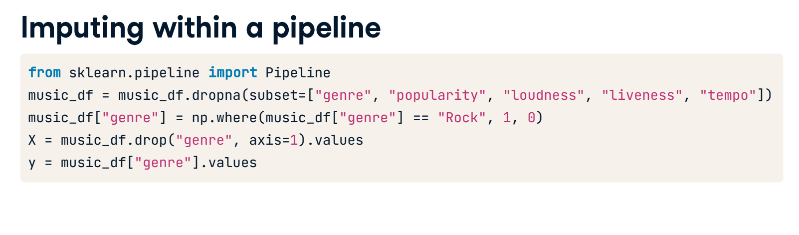
- Convert music_df["genre"] to values of 1 if the row contains "Rock", otherwise change the value to 0.
print(music_df.isna().sum().sort_values())

# Remove values where less than 5% are missing
music_df = music_df.dropna(subset=["genre", "popularity", "loudness", "liveness", "tempo"])

# Convert genre to a binary feature
music_df["genre"] = np.where(music_df["genre"] == "Rock", 1, 0)

print(music_df.isna().sum().sort_values())
print("Shape of the `music_df`: {}".format(music_df.shape))
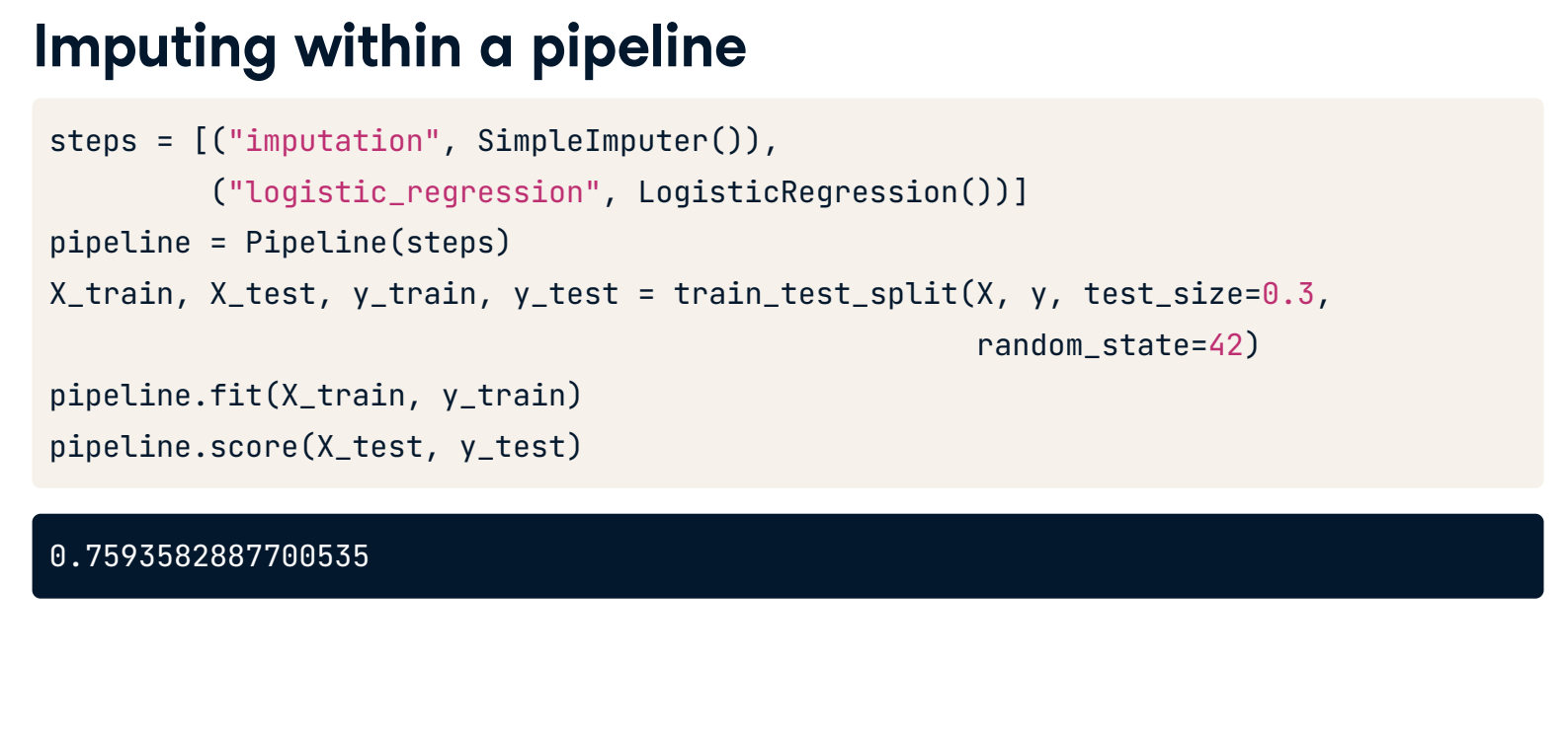
Pipeline for song genre prediction: I
Now it's time to build a pipeline. It will contain steps to impute missing values using the mean for each feature and build a KNN model for the classification of song genre.
The modified music_df dataset that you created in the previous exercise has been preloaded for you, along with KNeighborsClassifier and train_test_split.
Instructions:
- Import SimpleImputer and Pipeline.
- Instantiate an imputer.
- Instantiate a KNN classifier with three neighbors.
- Create steps, a list of tuples containing the imputer variable you created, called "imputer", followed by the knn model you created,
from sklearn.pipeline import Pipeline
from sklearn.impute import SimpleImputer
from sklearn.neighbors import KNeighborsClassifier
from sklearn.metrics import confusion_matrix

# Instantiate an imputer
imputer = SimpleImputer(strategy="most_frequent")

# Instantiate a knn model
knn = KNeighborsClassifier(n_neighbors=3)

# Build steps for the pipeline
steps = [("imputer", imputer),
         ("knn", knn)]
Pipeline for song genre prediction: II
Having set up the steps of the pipeline in the previous exercise, you will now use it on the music_df dataset to classify the genre of songs. What makes pipelines so incredibly useful is the simple interface that they provide.
X_train, X_test, y_train, and y_test have been preloaded for you, and confusion_matrix has been imported from sklearn.metrics.
Instructions:
- Create a pipeline using the steps you previously defined.
- Fit the pipeline to the training data.
- Make predictions on the test set.
- Calculate and print the confusion matrix.
imp_mean = SimpleImputer(strategy="mean")
steps = [("imputer", imp_mean),
        ("knn", knn)]

# Create the pipeline
pipeline = Pipeline(steps)

# Fit the pipeline to the training data
pipeline.fit(X_train, y_train)

# Make predictions on the test set
y_pred = pipeline.predict(X_test)

# Print the confusion matrix
print(confusion_matrix(y_test, y_pred))
Centering and scaling
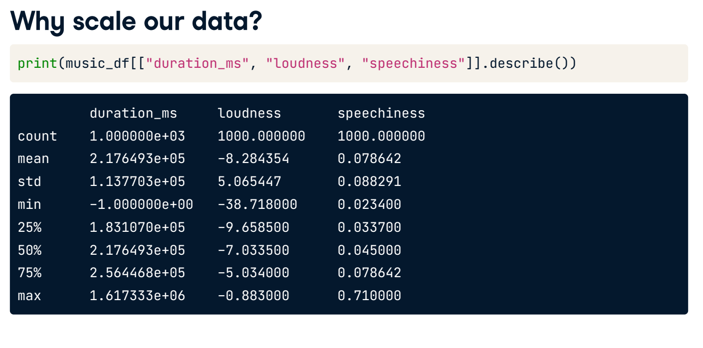
Why scale our data?
- Many models use some form of distance to inform them
- Features on larger scales can disproportionately influence the model
- Example: KNN uses distance explicitly when making predictions
- We want features to be on a similar scale
- Normalizing or standardizing (scaling and centering)
How to scale our data
- Subtract the mean and divide by variance
- All features are centered around zero and have a variance of one
- This is called standardization
- Can also subtract the minimum and divide by the range
- Minimum zero and maximum one
- Can also normarmalize so the data ranges from -1 to +1
- See scikit-learn docs for further details
Scaling in scikit-learn
from sklearn.preprocessing import StandardScaler

X = music_df.drop("genre", axis=1).values
y = music_df["genre"].values

X_train, X_test, y_train, y_test = train_test_split(X, y, test_size=0.2, random_state=42)

scaler = StandardScaler()

X_train_scaled = scaler.fit_transform(X_train)
X_test_scaled = scaler.transform(X_test)

print(np.mean(X), np.std(X))
print(np.mean(X_train_scaled), np.std(X_train_scaled))
Scaling in a pipeline
steps = [('scaler', StandardScaler()),('knn', KNeighborsClassifier(n_neighbors=6))]
pipeline = Pipeline(steps)

X_train, X_test, y_train, y_test = train_test_split(X, y, test_size=0.2, random_state=21)

knn_scaled = pipeline.fit(X_train, y_train)
y_pred = knn_scaled.predict(X_test)
print(knn_scaled.score(X_test, y_test))
Comparing performance using unscaled data
X_train, X_test, y_train, y_test = train_test_split(X, y, test_size=0.2, random_state=21)
knn_unscaled = KNeighborsClassifier(n_neighbors=6).fit(X_train, y_train)
print(knn_unscaled.score(X_test, y_test))
CV and scaling in a pipeline
from sklearn.model_selection import GridSearchCV

steps = [('scaler', StandardScaler()),('knn', KNeighborsClassifier())]

pipeline = Pipeline(steps)
parameters = {"knn__n_neighbors": np.arange(1, 50)}
X_train, X_test, y_train, y_test = train_test_split(X, y, test_size=0.2,random_state=21)

cv = GridSearchCV(pipeline, param_grid=parameters)
cv.fit(X_train, y_train)
y_pred = cv.predict(X_test)
Centering and scaling for regression (Exercise)
Now you have seen the benefits of scaling your data, you will use a pipeline to preprocess the music_df features and build a lasso regression model to predict a song's loudness.
X_train, X_test, y_train, and y_test have been created from the music_df dataset, where the target is "loudness" and the features are all other columns in the dataset. Lasso and Pipeline have also been imported for you.
Note that "genre" has been converted to a binary feature where 1 indicates a rock song, and 0 represents other genres.
Instructions:
- Import StandardScaler.
- Create the steps for the pipeline object, a StandardScaler object called "scaler", and a lasso model called "lasso" with alpha set to 0.5.
- Instantiate a pipeline with steps to scale and build a lasso regression model.
- Calculate the R-squared value on the test data.
from sklearn.preprocessing import StandardScaler
from sklearn.linear_model import Lasso

# Create pipeline steps
steps = [("scaler", StandardScaler()),
         ("lasso", Lasso(alpha=0.5))]

# Instantiate the pipeline
pipeline = Pipeline(steps)
pipeline.fit(X_train, y_train)

# Calculate and print R-squared
print(pipeline.score(X_test, y_test))
Centering and scaling for classification (Exercise)
Now you will bring together scaling and model building into a pipeline for cross-validation.
Your task is to build a pipeline to scale features in the music_df dataset and perform grid search cross-validation using a logistic regression model with different values for the hyperparameter C. The target variable here is "genre", which contains binary values for rock as 1 and any other genre as 0.
StandardScaler, LogisticRegression, and GridSearchCV have all been imported for you.
Instructions:
- Build the steps for the pipeline: a StandardScaler() object named "scaler", and a logistic regression model named "logreg".
- Create the parameters, searching 20 equally spaced float values ranging from 0.001 to 1.0 for the logistic regression model's C hyperparameter within the pipeline.
- Instantiate the grid search object.
- Fit the grid search object to the training data.
from sklearn.linear_model import LogisticRegression
from sklearn.model_selection import GridSearchCV

# Build the steps
steps = [
            ("scaler", StandardScaler()),
            ("logreg", LogisticRegression())
         ]
pipeline = Pipeline(steps)

# Create the parameter space
parameters = {"logreg__C": np.linspace(0.001, 1.0, 20)}
X_train, X_test, y_train, y_test = train_test_split(X, y, test_size=0.2,
                                                    random_state=21)

# Instantiate the grid search object
cv = GridSearchCV(pipeline, param_grid=parameters)

# Fit to the training data
cv.fit(X_train, y_train)
print(cv.best_score_, "\n", cv.best_params_)
Evaluating multiple models
Different models for different problems
Some guiding principles
Size of the dataset
- Fewer features = simpler model, faster training time
- Some models require large amounts of data to perform well
Interpretability
- Some models are easier to explain, which can be important for stakeholders
- Linear regression has high interpretability, as we can understand the coefficients
Flexibility
- May improve accuracy, by making fewer assumptions about data
- KNN is a more flexible model, doesn't assume any linear relationships
It's all in the metrics
Regression model performance:
- RMSE
- R-squared
Classification model performance:
- Accuracy
- Confusion matrix
- Precision, recall, F1-score
- ROC AUC
Train several models and evaluate performance out of the box
A note on scaling
- Models a(ected by scaling:
- KNN
- Linear Regression (plus Ridge, Lasso)
- Logistic Regression
- Artificial Neural Network
- Best to scale our data before evaluating models
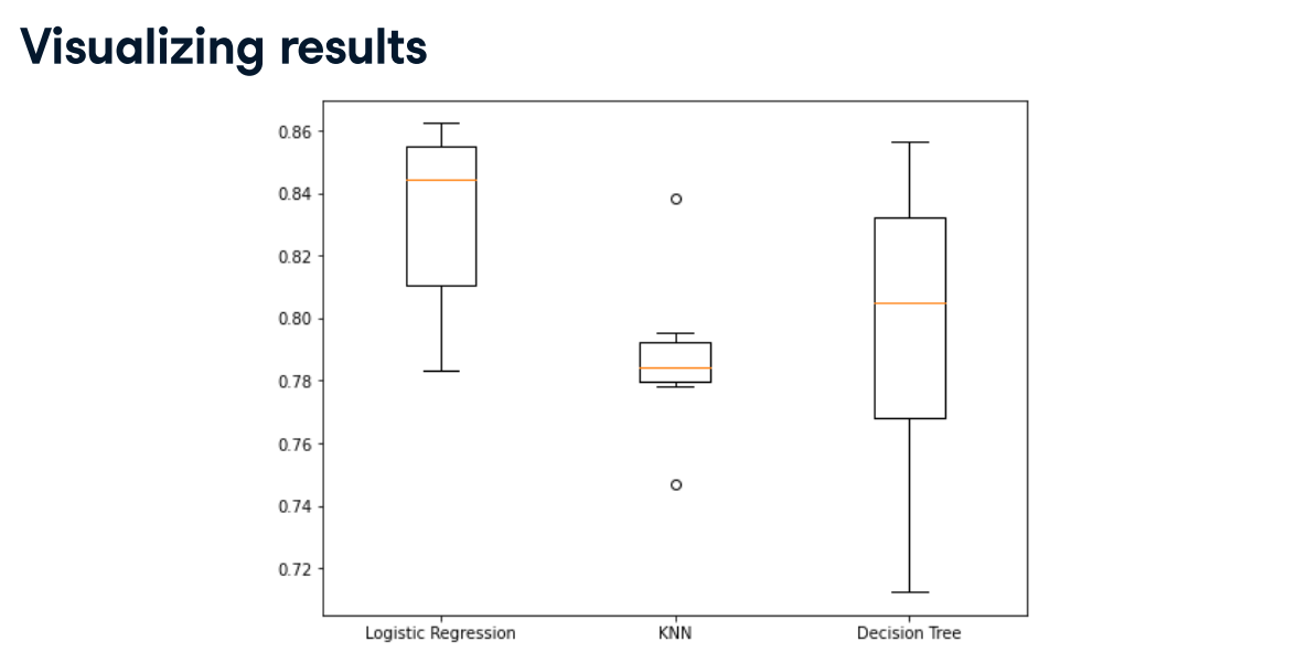
Evaluating classification models
import matplotlib.pyplot as plt
from sklearn.preprocessing import StandardScaler
from sklearn.model_selection import cross_val_score, KFold, train_test_split
from sklearn.neighbors import KNeighborsClassifier
from sklearn.linear_model import LogisticRegression
from sklearn.tree import DecisionTreeClassifier

X = music.drop("genre", axis=1).values
y = music["genre"].values
X_train, X_test, y_train, y_test = train_test_split(X, y, random_state=42)
scaler = StandardScaler()
X_train_scaled = scaler.fit_transform(X_train)
X_test_scaled = scaler.transform(X_test)
Evaluating classification models
models = {
            "Logistic Regression": LogisticRegression(),
            "KNN": KNeighborsClassifier(),
            "Decision Tree": DecisionTreeClassifier()
        }

results = []
for model in models.values():
    kf = KFold(n_splits=6, random_state=42, shuffle=True)
    cv_results = cross_val_score(model, X_train_scaled, y_train, cv=kf)
    results.append(cv_results)
plt.boxplot(results, labels=models.keys())
plt.show()
Visualizing regression model performance (Exercise)
Now you have seen how to evaluate multiple models out of the box, you will build three regression models to predict a song's "energy" levels.
The music_df dataset has had dummy variables for "genre" added. Also, feature and target arrays have been created, and these have been split into X_train, X_test, y_train, and y_test.
The following have been imported for you: LinearRegression, Ridge, Lasso, cross_val_score, and KFold.
Instructions:
- Write a for loop using model as the iterator, and model.values() as the iterable.
- Perform cross-validation on the training features and the training target array using the model, setting cv equal to the KFold object.
- Append the model's cross-validation scores to the results list.
- Create a box plot displaying the results, with the x-axis labels as the names of the models.
models = {
            "Linear Regression": LinearRegression(),
            "Ridge": Ridge(alpha=0.1),
            "Lasso": Lasso(alpha=0.1)
            }
results = []

# Loop through the models' values
for model in models.values():
  kf = KFold(n_splits=6, random_state=42, shuffle=True)

  # Perform cross-validation
  cv_scores = cross_val_score(model, X_train, y_train, cv=kf)

  # Append the results
  results.append(cv_scores)

# Create a box plot of the results
plt.boxplot(results, labels=models.keys())
plt.show()
Predicting on the test set (Exercise)
In the last exercise, linear regression and ridge appeared to produce similar results. It would be appropriate to select either of those models; however, you can check predictive performance on the test set to see if either one can outperform the other.
You will use root mean squared error (RMSE) as the metric. The dictionary models, containing the names and instances of the two models, has been preloaded for you along with the training and target arrays X_train_scaled, X_test_scaled, y_train, and y_test.
Instructions:
- Import mean_squared_error.
- Fit the model to the scaled training features and the training labels.
- Make predictions using the scaled test features.
- Calculate RMSE by passing the test set labels and the predicted labels.
from sklearn.metrics import mean_squared_error

for name, model in models.items():

  # Fit the model to the training data
  model.fit(X_train_scaled, y_train)

  # Make predictions on the test set
  y_pred = model.predict(X_test_scaled)

  # Calculate the test_rmse
  test_rmse = mean_squared_error(y_test, y_pred, squared=False)
  print("{} Test Set RMSE: {}".format(name, test_rmse))
Visualizing classification model performance (Exercise)
In this exercise, you will be solving a classification problem where the "popularity" column in the music_df dataset has been converted to binary values, with 1 representing popularity more than or equal to the median for the "popularity" column, and 0 indicating popularity below the median.
Your task is to build and visualize the results of three different models to classify whether a song is popular or not.
The data has been split, scaled, and preloaded for you as X_train_scaled, X_test_scaled, y_train, and y_test. Additionally, KNeighborsClassifier, DecisionTreeClassifier, and LogisticRegression have been imported.
Instructions:
- Create a dictionary of "Logistic Regression", "KNN", and "Decision Tree Classifier", setting the dictionary's values to a call of each model.
- Loop through the values in models.
- Instantiate a KFold object to perform 6 splits, setting shuffle to True and random_state to 12.
- Perform cross-validation using the model, the scaled training features, the target training set, and setting cv equal to kf.
models = {"Logistic Regression": LogisticRegression(),
          "KNN": KNeighborsClassifier(),
          "Decision Tree Classifier": DecisionTreeClassifier()}
results = []

# Loop through the models' values
for model in models.values():

  # Instantiate a KFold object
  kf = KFold(n_splits=6, random_state=12, shuffle=True)

  # Perform cross-validation
  cv_results = cross_val_score(model, X_train_scaled, y_train, cv=kf)
  results.append(cv_results)
plt.boxplot(results, labels=models.keys())
plt.show()
Pipeline for predicting song popularity (Exercise)
For the final exercise, you will build a pipeline to impute missing values, scale features, and perform hyperparameter tuning of a logistic regression model. The aim is to find the best parameters and accuracy when predicting song genre!
All the models and objects required to build the pipeline have been preloaded for you.
Instructions:
- Create the steps for the pipeline by calling a simple imputer, a standard scaler, and a logistic regression model.
- Create a pipeline object, and pass the steps variable.
- Instantiate a grid search object to perform cross-validation using the pipeline and the parameters.
- Print the best parameters and compute and print the test set accuracy score for the grid search object.
steps = [("imp_mean", SimpleImputer()),
         ("scaler", StandardScaler()),
         ("logreg", LogisticRegression())]

# Set up pipeline
pipeline = Pipeline(steps)
params = {"logreg__solver": ["newton-cg", "saga", "lbfgs"],
         "logreg__C": np.linspace(0.001, 1.0, 10)}

# Create the GridSearchCV object
tuning = GridSearchCV(pipeline, param_grid=params)
tuning.fit(X_train, y_train)
y_pred = tuning.predict(X_test)

# Compute and print performance
print("Tuned Logistic Regression Parameters: {}, Accuracy: {}".format(tuning.best_params_, tuning.score(X_test, y_test)))
What you've covered
- Using supervised learning techniques to build predictive models
- For both regression and classi,cation problems
- Underfitting and overfittng
- How to split data
- Cross-validation
- Data preprocessing techniques
- Model selection
- Hyperparameter tuning
- Model performance evaluation
- Using pipelines